Conditional formatting using multiple conditions - Excel 2007

Today I had a requirement to colour code in Excel based on a few conditions. At first I thouhgt I could use thre to four rules in the conditional formatting to achieve this result but when I did that the results that I was getting was not very satisfactory. So I thought I would try the And function of excel in conjunction with the conditional formatting and it worked wonders.

I wanted the entire row to be highlighted in a certain colour based on three conditions.

Here are the steps I followed to achieve what I was after.

• Select all the data that you want to colour code.
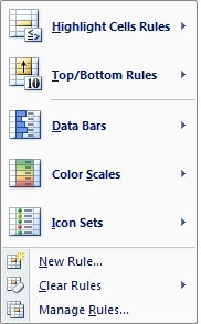
• Click on Conditional Formating on the Home Tab
• Choose Manage Rules as shown below
  

• From the dialog that appears click New Rule.
• Add the multiple conditions using the And function in the formula box
• The most important thing you need to do when you are adding the formula to highlight rows is to remove the $ sign that gets assigned when you choose the cell for entering a formula with a mouse.
• Choose the colour by clicking the format button and click ok
• Click Ok again to come out of the Manage Rules window.

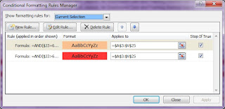
As you can see below I have added two rules and it is giving me the result that I want.